What I Learned in Machine Learning: From Dataset to Robust Decision
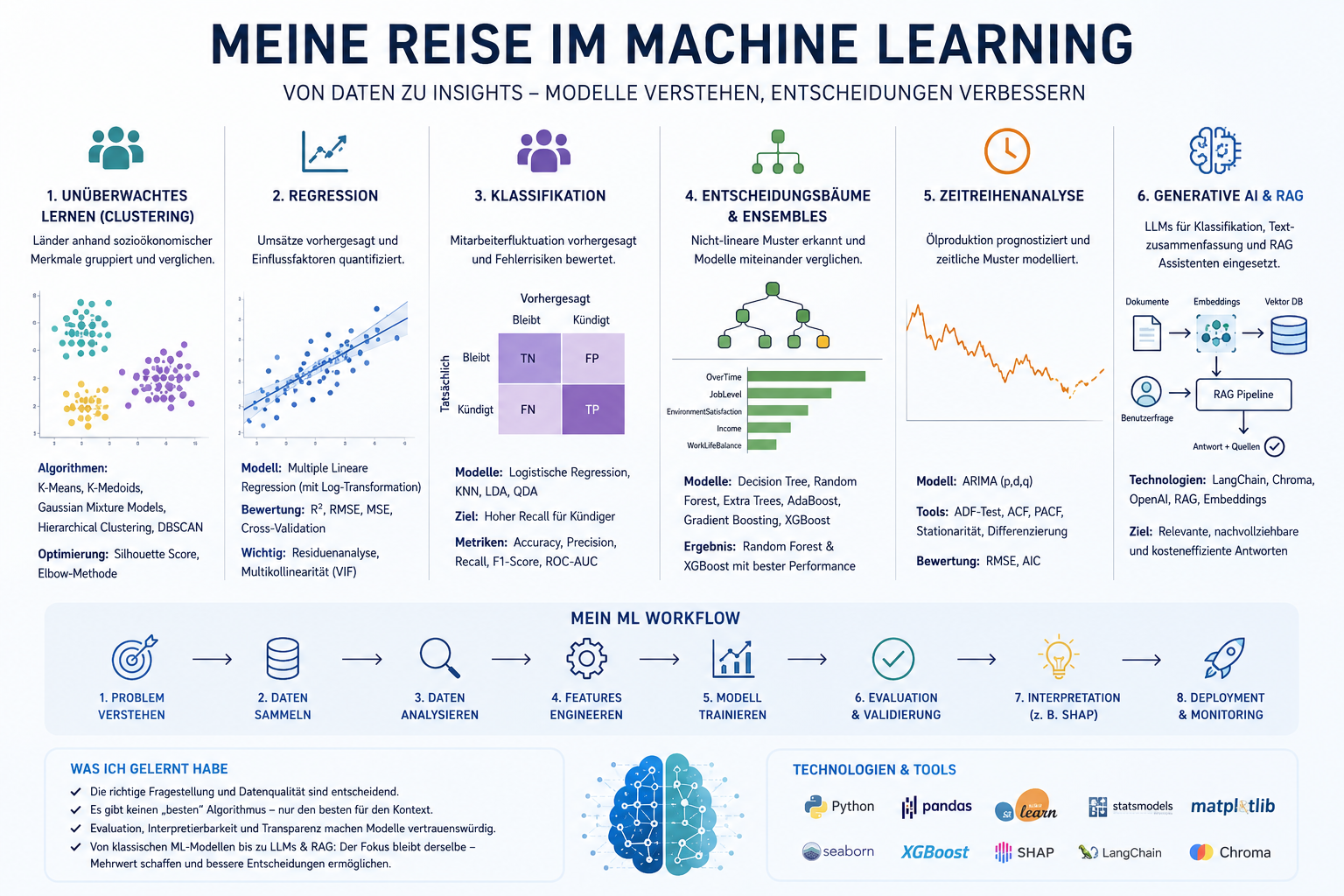
In my MIT further education in Applied AI & Data Science, I applied Machine Learning from the ground up using practical projects: from clustering, regression, and classification to Random Forest, XGBoost, and time series analysis, all the way to Generative AI and RAG. In this article, I show what I learned about data quality, model selection, evaluation, interpretability, and the journey from a notebook to a robust decision.
During my further education in Applied AI & Data Science at MIT, I got to know Machine Learning not just as a collection of various algorithms. It was crucial for me to understand the entire process: from a business question, through data analysis and modeling, to the evaluation, interpretation, and practical use of a model.
I worked with very diverse problems: grouping countries by socioeconomic characteristics, forecasting product sales, identifying employee attrition, comparing different ensemble models, and estimating future oil production based on historical time series. Later, Generative AI and Retrieval-Augmented Generation, or RAG for short, added another perspective.
The most important insight from this is: A powerful algorithm alone does not make a good Machine Learning solution.
Machine Learning Doesn't Start With the Model
Before I delved more deeply into Machine Learning, my focus as a software developer was naturally heavily on technical implementation. In the ML context, I learned that the actual work begins much earlier.
First, it must be clear:
- What real problem needs to be solved?
- What data is available?
- What exactly should be predicted or detected?
- Which incorrect decision would be particularly costly?
- How can the success of the model be meaningfully measured?
These questions determine whether a problem should be treated as regression, classification, clustering, or time series forecasting. They also determine which evaluation metric is important.
For a sales forecast, for example, the interest lies in how far the predicted values deviate from the actual sales. For predicting employee attrition, on the other hand, it is crucial to overlook as few actual at-risk employees as possible.
This helped me understand that technical modeling must always start from the business objective – not the other way around.
Understand Data Before Using It
A large part of the work in the notebooks consisted of exploratory data analysis, data cleaning, and preparation. This was one of the most important practical lessons for me.
Among other things, I learned to:
- identify and meaningfully handle missing values,
- remove unusable identifiers and constant variables,
- standardize inconsistent categories,
- analyze outliers and skewed distributions,
- scale numerical variables,
- encode categorical variables for models,
- investigate correlations,
- avoid data leakage between training and test sets.
It became clear that missing values should not simply be universally replaced with any average. In the BigMart project, for instance, relationships between product, location, and store characteristics were used to fill in missing values more plausibly.
Equally important was the realization that while data can show a statistical relationship, this is not automatically causal. High product visibility, for example, may be associated with lower sales figures because poorly performing products were subsequently placed more prominently. Visibility, then, isn't necessarily the cause of poor sales.
Machine Learning therefore requires not only programming skills but also critical thinking.
Unsupervised Learning: Identifying Structures Without a Known Target Variable
In the clustering project, I worked with socioeconomic data from various countries. Unlike classification, there was no predefined target variable. The model itself had to find groups of countries that were similar in terms of child mortality, income, life expectancy, inflation, healthcare expenditure, fertility, as well as imports and exports.
I compared several clustering methods:
- K-Means
- K-Medoids
- Gaussian Mixture Models
- hierarchical clustering
- DBSCAN
Before clustering, the features had to be standardized. Without scaling, variables with large numerical values, such as income, would have influenced the distance calculation more strongly than variables with smaller value ranges.
To select the number of clusters, I used the Elbow method and the Silhouette Score. Since the Elbow plot did not show a clear result, the Silhouette Score provided an additional basis for decision. For K-Means, three meaningfully distinguishable groups emerged.
The comparison of algorithms was particularly interesting for me. K-Means forms clusters around calculated centroids. K-Medoids, on the other hand, uses actual existing data points as centers, making it potentially more robust to extreme values. Gaussian Mixture Models treat group membership probabilistically, while DBSCAN identifies dense regions and can mark conspicuous points as noise or outliers.
The most important lesson here was: There is no inherently best clustering algorithm. The choice depends on the data structure, existing outliers, and the business objective. In this specific example, K-Medoids provided particularly clearly demarcated country groups.
Regression: Predicting Numerical Values and Explaining Relationships
In the BigMart project, the goal was to predict the sales of a product in a specific branch. A multiple linear regression model was developed for this.
I learned that linear regression is much more than just calling a fit() function. A robust regression model relies on various statistical assumptions.
These include, in particular:
- a sufficiently linear relationship,
- independent errors,
- a possibly constant error variance,
- sensibly distributed residuals,
- no problematic multicollinearity between the input variables.
To investigate multicollinearity, the Variance Inflation Factor was used. Non-significant or highly redundant variables were progressively removed. This made the model simpler and more interpretable without losing its essential predictive power.
Analyzing the residuals was particularly instructive. The initial model showed a discernible pattern in the errors. The assumptions of linear regression were thus not satisfactorily met. By applying a logarithmic transformation to the sales variable, this problem could be significantly reduced.
At the same time, the coefficient of determination (R²) improved from approximately 0.56 to around 0.72. The model could thus explain a significantly larger proportion of the sales differences.
I used various metrics for evaluation:
- R² to measure the explained variance,
- MSE for the average evaluation of squared errors,
- RMSE to represent the error in a more easily interpretable unit,
- Cross-Validation to check the generalization capability.
The similar R² value in cross-validation showed that the final model didn't only work on the training data.
I learned that transformations, statistical diagnostics, and residual analysis are not academic side topics. They determine whether the results of a model can be trustworthily interpreted at all.
Classification: Not Every Error Is Equally Important
The employee attrition project aimed to predict which employees were likely to leave the company.
The dataset was imbalanced: only approximately 16 percent of observations belonged to the class of attriting employees. A model that classified almost everyone as loyal could therefore achieve high accuracy yet be commercially worthless.
Here I learned to evaluate the types of classification errors from a business perspective.
A False Positive means that a loyal employee is incorrectly identified as at-risk. The company might unnecessarily offer them measures or incentives.
A False Negative is more critical in this scenario: The model fails to identify an employee who is actually at-risk. The company might lose a valuable skilled worker without being able to react in time.
Therefore, the Recall of the positive class was chosen as the central target metric.
I initially worked with:
- a dummy model as a baseline,
- logistic regression,
- K-Nearest Neighbors,
- Linear Discriminant Analysis,
- Quadratic Discriminant Analysis.
The dummy model was important because a real model must not just be "somehow good," but must demonstrably surpass a simple baseline value.
With K-Nearest Neighbors, I also learned about the influence of scaling and hyperparameters. The number of neighbors, the distance metric, and the weighting were optimized using GridSearchCV, among other methods.
At the same time, the project showed that high recall does not automatically mean a perfect model. The optimized KNN model achieved strong recall but showed signs of overfitting. Such a result must be transparently stated and further investigated.
Explainable AI with SHAP
A model should not just deliver a prediction. Especially for decisions involving people, it must be comprehensible which features influenced the prediction.
For this, I used SHAP. With SHAP values, I could analyze both the global importance of the features and the reasons for individual predictions.
In the attrition model, the following factors were among the important influencing variables:
- overtime,
- marital status,
- job satisfaction,
- work-life balance,
- income,
- professional experience and work engagement.
Overtime proved to be a particularly strong driver of predicted attrition. Very high job satisfaction, conversely, reduced the probability of resignation.
It was important for me to understand that feature importance and SHAP values do not prove causality. They explain how the model makes its decisions. They do not automatically show that a feature is the real cause of a behavior.
Nevertheless, such explanations are crucial for testing models, discussing them professionally, and making them transparent to stakeholders.
Decision Trees, Random Forest, and Boosting
In the next step, the attrition problem was investigated using tree-based methods.
A single decision tree is easy to understand. It makes predictions through a sequence of comprehensible rules. At the same time, a large, unrestricted tree strongly tends towards overfitting: it can almost memorize the training data but generalizes poorly to new data.
Therefore, I learned to regulate decision trees using parameters such as:
- maximum tree depth,
- minimum number of observations per leaf,
- splitting criterion,
- class weights.
Subsequently, various ensemble methods were compared:
- Random Forest
- Extra Trees
- AdaBoost
- Gradient Boosting
- XGBoost
Random Forest combines many decision trees trained on different data and feature subsets. This reduces the dependence on a single unstable tree.
Boosting takes a different approach: the models are built iteratively, with new models responding particularly to the errors of previous models.
In the results, the optimized Random Forest and XGBoost achieved the strongest combinations of Recall, Precision, and Accuracy. The optimized Random Forest achieved the highest Recall, while XGBoost achieved very similar detection performance with high Precision and Accuracy.
However, the crucial lesson for me was not that Random Forest or XGBoost are fundamentally "better." I learned to systematically compare models and evaluate their strengths based on the specific business objective.
A more complex model is only an improvement if its additional benefit justifies the loss of simplicity and interpretability.
Time Series: The Past Is Not Simply a Normal Dataset
When forecasting oil production, I got to know a completely different form of modeling.
Time series data have a natural order. Therefore, training and test data must not be randomly shuffled. The model must be trained on the past and tested at later points in time.
I dealt with:
- Trend and time series decomposition,
- Stationarity,
- Augmented Dickey-Fuller Test,
- Differencing,
- Autocorrelation,
- ACF and PACF plots,
- AR, MA, ARMA, and ARIMA models.
The original time series was non-stationary. Its statistical behavior changed over time. Only after third-order differencing did the ADF test achieve a sufficiently small p-value.
Using ACF and PACF, it was possible to investigate how strongly today's values relate to earlier observations or earlier errors. Based on this, different combinations of the ARIMA parameters p, d, and q were tested.
For model evaluation, AIC and RMSE were compared. Both metrics pursue different goals:
RMSE evaluates the magnitude of forecast errors. AIC additionally considers model complexity and penalizes unnecessarily complicated models.
In the notebook, ARIMA(2,3,2) provided the best result based on RMSE. Auto-ARIMA, on the other hand, suggested a different model as it primarily optimized AIC.
That was a particularly valuable insight: Even automated model selection is not objectively detached from the goal. The result depends on which metric the search process optimizes.
From Classical Machine Learning to Generative AI and RAG
The Generative AI notebook supplemented the classical Machine Learning topics with three practical applications:
- Classification of hotel reviews,
- Creation of patient-friendly medical summaries,
- Development of a RAG-based assistant for HR policies.
No classical model was trained from scratch. Instead, an existing Large Language Model, Prompt Engineering, Embeddings, and a vector database were used.
For the HR assistant, I implemented a complete RAG pipeline in Python:
- Read PDF documents,
- Tokenize text into overlapping, token-based chunks,
- Generate embeddings,
- Persistently store the vectors in Chroma,
- Retrieve relevant text sections via semantic similarity,
- Pass the found content as context to the LLM,
- Generate a response based solely on these sources.
Additionally, sources or chunk IDs were returned. If the information was not available in the document, the system was explicitly instructed to state that it did not know the answer.
Here, I could transfer much from classical Machine Learning: Data quality, evaluation, reproducible results, error analysis, and the necessity of a baseline do not disappear with Generative AI. They become even more important because LLM outputs are probabilistic and not always reliable.
Cost control also played a practical role. I worked with tight token limits, clearly defined output formats, and controlled parameters. For classifications, for example, the model should only output a single valid label. Structured answers, limited output lengths, and specifically curated context reduce both costs and sources of error.
How These Projects Changed My Way of Thinking
Through these projects, I gained practical experience with a complete ML workflow:
- Translating business problems into analyzable tasks,
- Examining and cleaning data,
- Selecting appropriate model families,
- Building baselines,
- Correctly splitting data into training and test sets,
- Optimizing hyperparameters,
- Identifying overfitting and underfitting,
- Selecting suitable metrics,
- Explaining results,
- Translating technical results into actionable recommendations.
My background in software development and quality assurance strongly influenced my view of Machine Learning. I see a model not as an isolated notebook, but as part of a larger system. This includes tests, data validation, versioning, reproducible pipelines, error handling, monitoring, documentation, and controlled integration into existing applications.
A model with a good score is far from a production-ready system.
My Honest Conclusion
I would not claim that a few months of further education replace several years of specialized production experience as a Data Scientist or ML Engineer. That would be neither credible nor professionally correct.
What I have built, however, is a solid and practically proven foundation. I can categorize different ML problems, analyze data, implement and compare multiple model classes, critically evaluate results, and recognize the limitations of a model.
Above all, I learned not to view Machine Learning as a magic black box. Behind every good solution are clear assumptions, clean data, conscious decisions, and honest evaluation.
For me, this connects my previous path as a software developer, QA specialist, project manager, and product owner with a new competence: the ability to assess data- and AI-based solutions not only in terms of technical implementation but also quality, benefit, risks, and long-term maintainability.